VISION

BY DAVID MARR

Published posthumously, this research monograph was seminal to the field of computational neuroscience. Marr delves into the human visual system, and showcases the computational neuroscience approach. This book was a pleasure to read and ended too soon. After reading, I implemented several of the algorithms described.

A short biography of David Marr

Buy the book from the publisher

The book begins by defining the purpose of the visual system, and Marr relates everything to this purpose: “Vision is the process of discovering from images what is present in the world, and where it is.”

Each section of the book states a problem to be solved and then analyses it at several levels. First, Marr looks at the computational theory: what is the goal to be accomplished and how to achieve it at an algorithmic level. Then, he looks at what information needs to be represented and how the inputs are transformed into the outputs. Finally, he looks at how the process can be realized physically, either by a computer or by the brain.

Inside of the Retina

The first stages of visual processing happen inside of the retina. The retina transmits a filtered image to the brain, not the raw light intensities. The retina detects light and then applies Mexican-hat shaped filters to it. The choice of Mexican-hat filter is well justified, both with theory and with biology. This filter responds to variations in the input, but not areas of constant intensity or linear gradients. Also it is only sensitive to input features that have a similar size as the filter. In the human retina, there are at least 4 four different sizes of Mexican-hat shaped filters which are sized at powers of two of each other, so the retina can detect features over a broad range of scales.

The retina also calculates the time derivative of the filtered image, which is used to detect motion.

These transforms preserve almost all of the incoming visual information and it is possible to mostly reconstruct the original image from the filtered outputs. The notable exception is that while the relative differences between pixels are preserved, the absolute magnitude of the image’s light intensity is lost.

For a more recent and in-depth review of the retina’s biology see: http://www.pnas.org/cgi/doi/10.1073/pnas.1011782107. However, it’s worth reading VISION first because that review does not attempt to explain the computations of the retina.

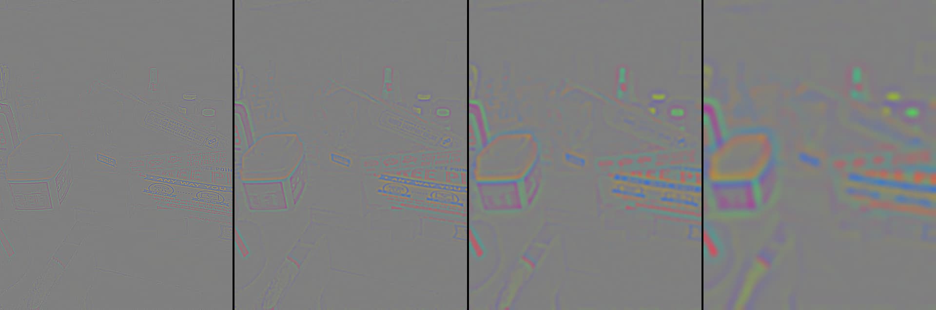
To demonstrate these transforms, I applied them to this test image:

Converted to greyscale and with 4 sizes of Mexican-hat filters applied:

Colors are processed by taking the difference between the color channels before applying the Mexican-hat filters. The retina subtracts (red - green) and (blue - yellow). Here is a false-color representation of the result:

I also experimented with contrast normalization, though the book does not cover this topic. Contrast normalization amplifies weak stimuli and weakens strong stimuli. This allows the retina represent a larger range of stimuli strengths with a smaller range of output values. It also causes the retina to encode the relative strengths of nearby stimuli because it normalizes large patches of the image. Adjacent stimuli attenuate each other.

My implementation was inspired by a prior model of the retina which also does contrast normalization:

Virtual Retina: A biological retina model and simulator, with contrast gain control
Adrien Wohrer & Pierre Kornprobst, 2009
DOI: 10.1007/s10827-008-0108-4
Website

Left: No Contrast Normalization | Right: With Contrast Normalization

Notice that with contrast normalization you can see the color of the pizza in the pizza box, more details on the cats face, and the light switch in the top-right corner. The faint stimuli are amplified by about 2x and yet the strong stimuli are not saturated.

The Primal Sketch

Moving into the brain, the next stage of processing seeks to understand the 2D image in a very literal way. The image is decomposed into primitive features, such as edges, lines, or blobs of color. Marr calls this the primal sketch. The purpose of these primitive tokens is to represent the aspects of the 2D image which correspond to the 3D structure of physical objects.

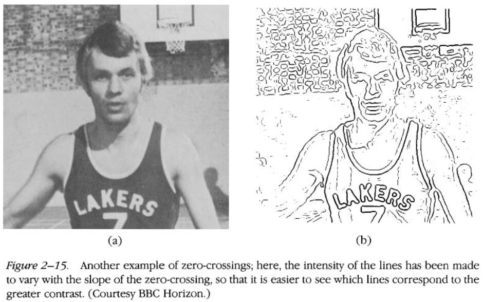
The most basic primitives are the “zero-crossings” in the retinal inputs. The zero crossings are caused by the Mexican-hat filters passing over sudden changes in light intensity. They are essentially a form of “edge detection”. At this point Marr discusses the nature of edges in 2D images versus in the 3D world. All (detectable) edges in the 3D world will have some kind of corresponding edge in the 2D image, and these 2D edges will almost certainly be visible at multiple scales. However there are also edges in the 2D image which do not correspond to an edge in the 3D world.

Then the zero crossings are built up into various larger tokens, such as line segments, curves, circular blobs, etc. Of particular importance are the terminations (end points) of line segments, because they are highly recognizable and can be located very precisely which makes them good features. In addition, these tokens can have a lot of associated information for example about the color, contrast, size, or orientation.

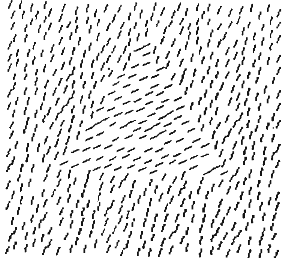
The brain groups together primitives which are similar to each other and in close proximity. These groups can form “virtual lines” where you perceive a line connecting the primitives, even though no line truly exists. They can also form “virtual edges” at the boundaries of the group. Groups of primitives are also primitive features which can be composed into larger groups, in a recursive fashion.

At this point we have detected all of the low-level 2D image features which we will use. The next stage of processing is to sort through the features and piece together an understanding of the physical surfaces which generated these image features.

Simple Cells

In 1958 Hubel and Weisel discovered “simple cells” which are neurons in the primary visual cortex (V1) that respond to edges. These cells appear to detect the zero crossings that Marr writes about. Since then more cells have been found in V1 which detect other features that Marr writes about.

The retina transmits positive and negative values using different axons. The retina contains two separate pathways for applying the Mexican-hat shaped filters for this purpose. This encoding scheme makes it very easy for downstream neurons to detect the zero crossings in the filtered image.

I used a spatial pooler to simulate the “simple cells” of the primary visual cortex; to detect the primitive features and to form the primal sketch.

I modified the spatial pooler algorithm to support rate-coded inputs, because the retina clearly generates them. I replaced the regular binary synapses with weighted synapses, and I replaced the learning rule with:

delta_weight = learning_rate * presynaptic_input * postsynaptic_activity

Notice that this rule will only increase the weights. After applying the learning rule the sum of synaptic weights to each cell is normalized to one. This implements the synaptic decrement for inactive synapses and this also controls the positive feed-back caused by hebbian learning.

Another key modification to the spatial pooler algorithm is to alter how it handles topology. The spatial pooler algorithm, as described by Numenta, has cells spread out over the input space and each of those cells has synapses to the nearby inputs. This allows the population of cells to cover the whole input space despite the fact that each cell has a small local receptive field. Instead I modified the spatial pooler to have a single set of cells which are repeated across at every location in the input space. This is the convolution trick borrowed from convolutional neural networks. The primary advantage of convolving a single set of cells across the image (instead of having different cells at each location) is that they will generate comparable output because they use the same synaptic weights. Given identical image patches, the convolved cells will have the same response.

I trained my modified spatial pooler on natural imagery. I used images from the documentary “Planet Earth, by David Attenborough”. The size of the cells’ receptive fields were 5 x 5 pixels.

Then, I reverse engineered the synaptic weights to find images which maximally activate each cell, and I found many cells that detect the features described by Marr, and experimentally found by Hubel and Weisel. In addition there are cells for a variety of different colors, sizes, and angles.

Cells that respond to edges:

Cells that respond to lines:

Cells that respond to line terminations:

Cells that respond to blobs:

There are also some cells that respond to miscellaneous/uncategorized inputs.